Excel-in-XL Intermediate

Excel-in-XL course:
Basic to Intermediate Level

Attendees knowledge of this course steps forward from Beginners level to Intermediate level user of Microsoft Excel.


WHO SHOULD ATTEND

This course is important for those who are using Excel as their basic working tool and want to step ahead by learning smart ways. After learning skills in this course and by efficiently use them can save at-least 4 to 5 hours weekly.

Beginner users who have basic knowledge of Excel and can make basic calculations.

WHAT YOU WILL BE ABLE TO DO

Environment:

• Better understanding of Excel 2016 interface
• Easily working around with Excel environment (e.g. rows/columns/etc, selections)
• Secure data and/or restrict your users to post data within required cells only.

Data & File Handling:

• Change the order of data
• View part of data based on criterias
• Reports Preparations (Data and Cell Formatting), 
• Page Setup, File handling and Printing.

Formulas: 
Formulas make Excel a smart spreadsheet program. In this course you will learn ...

• Fundamentals of formulas and functions. 
• Simple and complex formulas introduction
• Cell Referencing, its types and their usages.
• Auto & quick SUMs, other basic functions.

Charts:

• Introduction to data visualization with Charts
• Ability of select appropriate chart, which is suitable for which data
• Create Column, Bar, Line and Pie graphs.
• Customization

Smart practical tips and tricks along-with shortcut keys.






To register yourself in upcomming sessions fill the below form for registration...
<...>
 

*int_v2*

Become Certified MOS 2016 (a YouTube PlayList)

Learn how to become certified Microsoft Office 2016 Specialist of Word, Excel, PowerPoint & Outlook / Expert of Word & Excel / Master from different experts.
.

.
Above video belongs to a PlayList
Collection of MOS 2016 Video Tutorials from experts

Data Validation - Basics

To prevent incorrect data posting in specific cells we use Data Validation. 
if you created a worksheet that will be used by others, you need to ensure that only correct data that matches with requirements is entered. 

For example: between (10 and 20), or only specific text (Mr., Mrs, or Miss), etc.

Following are some basic data validations:

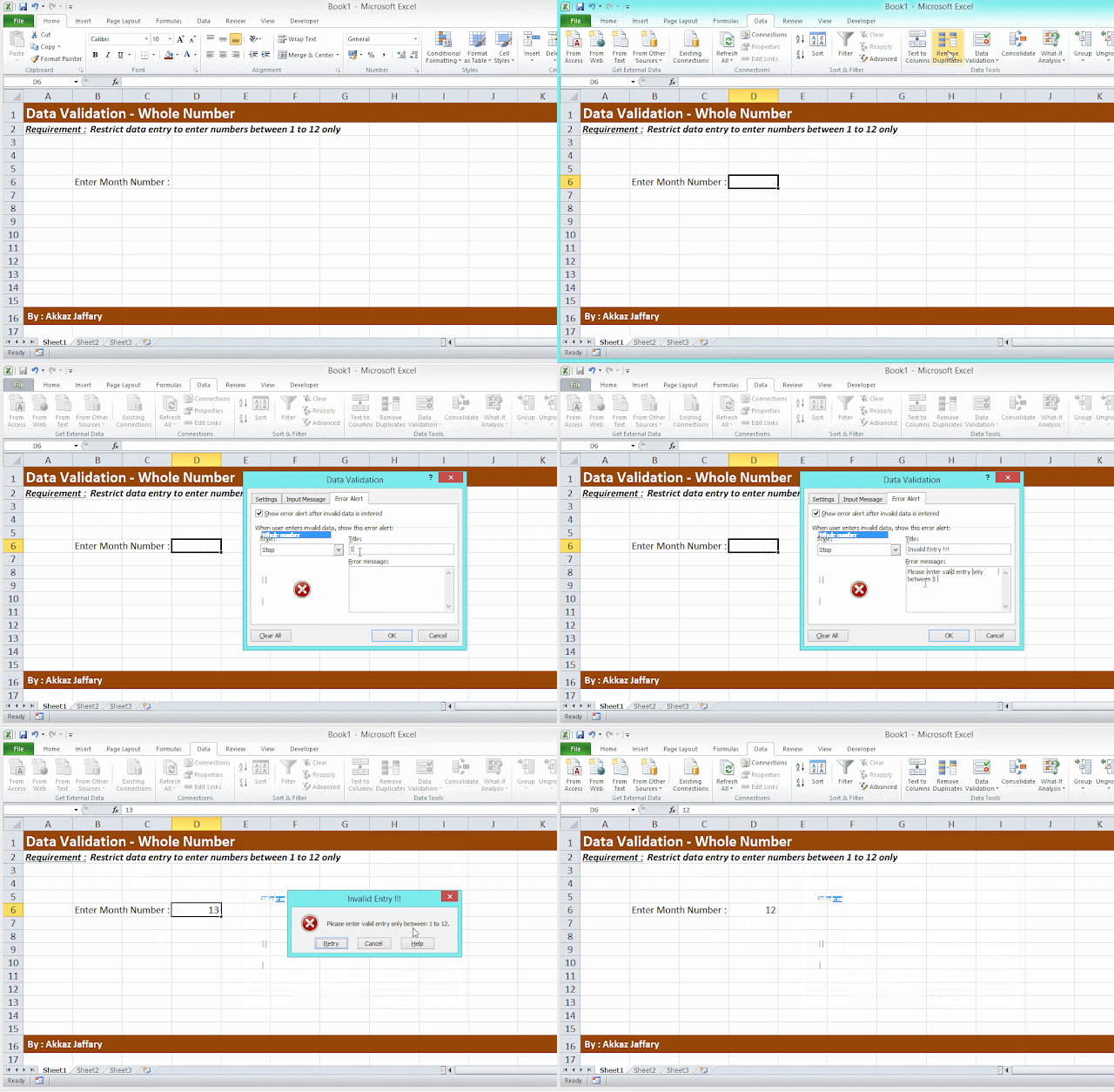
Whole Number:This can be used to restrict whole number data entry as per defined validation only.
For example you can prevent data which is out of a number range. See below animation.

If you understand the above, you can explore following more options to validate the data entery:

* Decimal
* Date
* Time
* Text Length
* List   (multi-choice drop-down list.  Items separated with comma)

Following advanced options and will be posted seperately ...

* Custom

For more detail, write us ...

Cell Styles

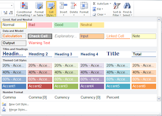
A smart way to quickly format a cell or range of cells is Cell Style. A cell style is a defined set of misc. formatting, such as fonts, font sizes, font Colors, number formats, cell borders, cell shading, etc.

Microsoft Office Excel has many predefined cell styles that you can apply. You can modify or duplicate a cell style to create your own, custom cell style as per your requirement or taste.

BENEFITS OF USING CELL STYLES:
* Apply Several formats in one step
* Ensure consistent formatting
* Saves time by just selecting a defined style.

Important: Cell styles are based on the document theme that is applied to the whole workbook. When you switch to another document theme, the cell styles are updated to match the new document theme.

APPLY CELL STYLE 
1. Select a cell or range of cells
2. Click on "Cell Styles" button at Home tab
3. click on a pre-defined cell style




CREATE NEW OWN STYLE
1. Goto Home tab > Styles group > Cell Styles
2. Click "New Cell Styles"
3. Type an appropriate name for the new cell style in Style name box.
4. Click on Format button
5. Format Cells dialogue box appears with many tabs, where from you can select different formats
6. After selection of format(s) click on OK button.
Now u can use/apply this new style.

MODIFY A STYLE
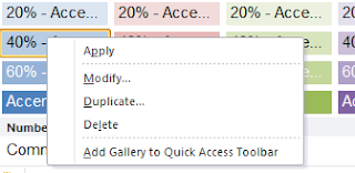
* To modify an existing cell style, right-click that cell style, and then click Modify.
* Cell Style Dialogue Box will appear
* Click on format button and change formatting as required




STYLE DERIVED FROM AN OLD STYLE (DUPLICATE)
* To create a style derived form an existing cell style, right-click that cell style, and then click Duplicate.
* Cell Style Dialogue Box will appear
* Change the style name
* Click on format button and change formatting as required

Note: A duplicate cell style and a renamed cell style are added to the list of custom cell styles. If you do not rename a built-in cell style, the built-in cell style will be updated with any changes that you make.


For more information; write us or check below link
Support.Office.Com

Formatting Shortcut Keys in Excel 2010

Formatting Shortcut Keys

SHORTCUT_KEYS____	DESCRIPTION______________________________________
Ctrl + B	Apply bold formatting on selected contents
Ctrl + I	Apply italic formatting on selected contents
Ctrl + U	Apply underline formatting on selected contents
Ctrl + 5	Apply/remove strike-through formatting on selected contents
Ctrl + 1	Open Format Cells dialog box
Alt  + ‘	Open Style dialog box
Ctrl + Shft + ~	Apply General Format on selected range
Ctrl + Shft + $	Apply Currency format on selected range
Ctrl + Shft + %	Apply Percentage format on selected range (#,###%)
Ctrl + Shft + #	Apply Date format on selected range (dd-mmm-yy)
Ctrl + Shft + @	Apply Time format on selected range (h:mm:ss AM/PM)
Ctrl + Shft + !	Apply Number format on selected range (#,###.00)
Ctrl + Shft + &	Apply outline-border on selected range
Ctrl + Shft + _	Remove cell borders from selected range
Alt + H + B + A	Apply cell border to all selected cells.

for more information, check below link:

Support.Office.Com

Pivot Table (Beginner)

PIVOT TABLES
 
Being able to quickly analyze data can help you make better business decisions.

When you have data especially large data, PivotTables are a great way to summarize, analyze, explore, and present it. PivotTables are highly flexible and can be quickly adjusted depending on how you need to display your results. You can also create PivotCharts based on PivotTables that will automatically update when your PivotTables do.

You can create PivotTable with just a few clicks, but before you get started be careful for …
* Data should be in tabular format
* All columns should have proper header at first row
* Not have any blank row or column
* Data types within a column should be same
* Excel tables are a great PivotTable data source, because rows or columns added to a table are automatically included in the PivotTable when you refresh the data. Otherwise, you need to manually update the data source range.
* PivotTables work on a snapshot of your data, called the cache, so your actual data doesn't get altered in any way.

GETTING STARTED

Create PivotTable: 
1. click anywhere in your source data
 

2. from Insert tab click at PivotTable button

3. Create PivotTable dialog box will be appeared. Review the selections, then click OK.

4. A blank PivotTable will be appeared on left side of your worksheet, and its field lists will be at right side.
 

Add fields to the PivotTable:

Example of PivotTable usage
1. Comparing Sales Totals of Different Products
2. Combine Duplicate Data

Our data consist of 500 rows and having 08 columns. InvNo, InvDate, Customer, City, Product, ProdCategory, QuantitySold, Amount

To see product wise sales, in PivotTable Fields pane add/drag fields as
* Product in Row area
* Amount in Values area
* ProdCategory in Filter area.

For more information, check below link or write us ...
Support.Office.com 

Repeat Last Command Used (Shortkey)

Repeat last command used by pressing <F4> key.

Shortkeys to work around in Excel Environment (Shortkeys/HotKeys)

Important short keys to work around in Microsoft Excel Environment to speedup your productivity ...  

KEYS------------------------	Description-------------------------------------------
Selection
Ctrl + A	Select All (if...)
Shft + ArrowKeys	Select adjacent cell
Shft + SpaceBar	Select whole row
Ctrl + SpaceBar	Select whole column
Column/ Rows/ Cells
Alt O C W	To change column width by points
Alt O R E	To change row height by points
Alt O C A	AutoFit column width as selected cell’s data.
Alt I R	Insert above a blank row
Alt I C	Insert right-side a blank column
Ctrl +	Insert column/ Row/ Cell.
Ctrl –	Delete column/ Row/ Cell.
Ctrl 0	Hide column(s)
Ctrl 9	Hide row(s)
Alt O C U	Unhide columns within selected range
Alt O R U	Unhide rows within selected range
Alt W F F	Toggle Freeze/ Unfreeze rows/columns
Sheets
Ctrl PgUp	Goto previous sheet
Ctrl PgDn	Goto next sheet
Shft F11	Insert new worksheet
Alt H O R	Rename active sheet
Alt T P P	Toggle Protect/ Unprotect sheet
Alt I B	Toggle page break
Alt H O M	To get “Copy and Move” dialogue box
While Cell Editing
Home	Goto start of line
Ctrl Home	Goto Start of cell contents
End	Goto end of line
Ctrl End	Goto end of cell contents
Ctrl LeftArrow	Move one word left side
Ctrl RigthArrow	Move one word right side
Ctrl Delete	To delete all data right side of cursor in cell.

CHOOSE Function

Returns a value from a list based on position. Uses index_num to return a value from arguments.

Syntax:     =CHOOSE(index_num, value1, [value2], ...)

index_num  must be a number or a formula or reference to a cell containing a number between 1 and 254.

value1, value2, ...  Value 1 is required, subsequent values are optional. 1 to 254 value arguments from which CHOOSE selects a value.


Examples:
if value1 through value7 are the days of the week, CHOOSE returns one of the days when a number between 1 and 7 is used as index_num.

=CHOOSE(A1,"Mon","Tue","Wed","Thu","Fri","Sat","Sun")

=SUM(CHOOSE(2,A1:A10,B1:B10,C1:C10))
this will work as =SUM(B1:B10)


Common Errors
#VALUE!    -  
*  The supplied index_num is less than 1 or is greater than the supplied number of values;
*  The supplied index_num argument is non-numeric.

#NAME?
*  Occurs if any of the value arguments are text values that are not enclosed in quotes and are not valid cell references.




For more detail, check below links or contact us ...
* CHOOSE Function at https://office.com

Microsoft Excel 2010 Interface

At first; Microsoft Excel 2010 interface (screen) looks as divided into two parts; 1) Command buttons and 2) Worksheet; but; there are many other parts as well, if you have knowledge about them you will have an ease to read and understand whenever they referred- in any process either downloaded from internet, book or even by a teacher.

Below is a snap along-with parts names. Click to enlarge.

.